In the previous article, I shared the basics of machine learning and its types in this article I will cover the most important and basic algorithm in machine learning ie Linear Regression... This is the type of supervised machine learning

Let's Start ,

How do Machine Learn?

As I mentioned in the previous article, the machine learns from data to find a pattern using machine Learning Algorithms this is the basic algorithm by which the machine learns.

Be ready to deep dive into the algorithm.

Linear Regression

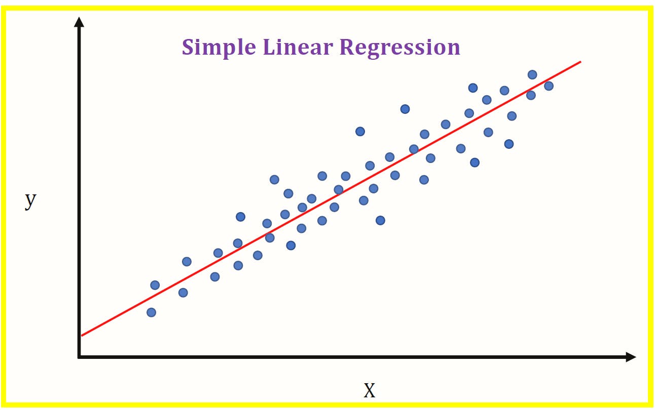
Let us break down the term into two "Linear" and "Regression" the first term linear refers to the line and Regression refers to the continuous value Let us combine now ,by using the line we are trying to predict the continuous value this what the overview of Linear Regression..

Let us see

How Linear Regression works?

what is the line equation?

the answer is Y=MX+C

here M=slope and C is intercept this is basic high school maths formula you may ask why are you asking this let me say , can you spot with value of X your finding the value of Y

Here Y is the target variable or dependent variable and X is the independent variable Y depends on X so it is called the dependent variable

But in real world, we cannot directly predict the value of y using only this equation because we have large amount of data ,we try to find the parameter with which when a new value is given as input we can find acurately.. here parameter refers to slope -M and intercept -C but how can we do this

Steps involved in linear regression:

1. First we randomly take the value of the parameter and form a line with the parameter

2. In the second step we try to find an error or residual which

   Error= Actual - Predicted

3. In the third step we try to change the parameter value such that the line forming with parameter will be the best fit line that fits the data linearly with less error.

Step 1

Take random parameter and form a line

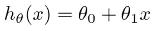
this equation is called Hypothesis or simply Line equation you may ask why hypothesis name came because the researchers coined the term hypothesis .This is same as line equation we saw above .

Step 2

Find an error or residual

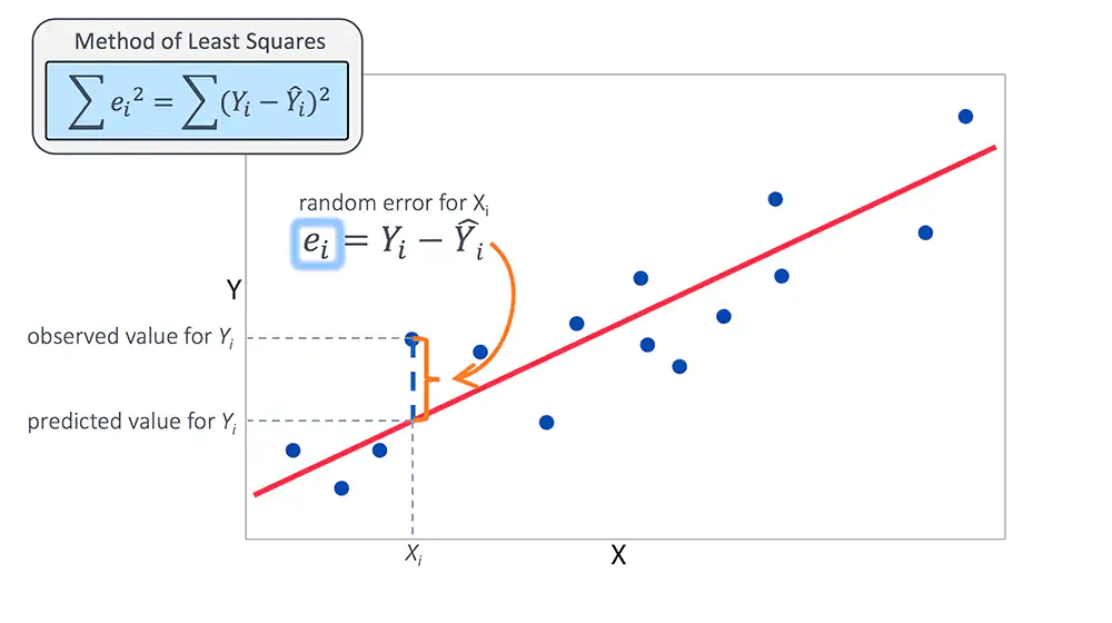
In the previous step we formed a random line which is not the best fit line inorder to form the best fit line we calculate the error through which we update the parameter. there some methods of calculating error like

1. Mean squared error

2. Mean Absolute error

3. Root Mean squared error

In this article we focus on Mean squared error this the formula

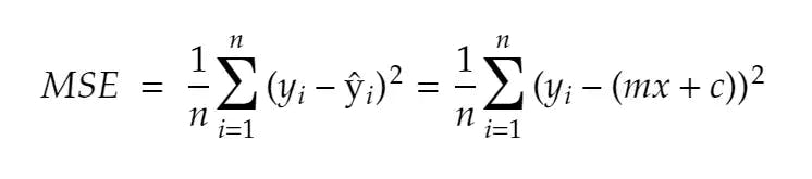
this is also called as cost function.

Step 3

Update the weights

One such method to update the weight is Gradient decent Algorithm,

Gradient Descent Algorithm (GDA)

GDA’s main objective is to minimize the cost function. Cost function h𝜽 helps us to figure out the best possible values for 𝜽0 and 𝜽1 which would provide the best fit line for the data points.

It is one of the best optimization algorithms to minimise errors (difference of actual value and predicted value). Using GDA we will figure out a minimal cost function by applying various parameters for 𝜽0 and 𝜽1 and see the slope intercept until it reaches convergence.

In other words → we start with some values for 𝜽0 and 𝜽1 and change these values iteratively to reduce the cost. Gradient descent helps us on how to change the values.

How it works?

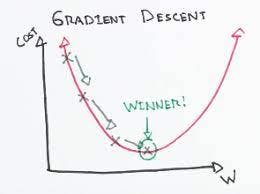
this is plot between cost function and weights. our task is to minimise cost function

take a step towards downward direction; from the each step, look out the direction again to get down faster and downhill quickly. Mathematically speaking:

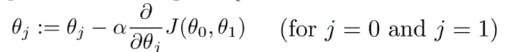
1. To update 𝜽0 and 𝜽1 we take gradients from the cost function. To find these gradients, we take partial derivatives with respect to 𝜽0 and 𝜽1 The partial derivatives are the gradients and they are used to update the values of 𝜽0 and 𝜽1 .

2. The number of steps taken is the learning rate (𝛼 below). This decides on how fast the algorithm converges to the minima. Alpha is the learning rate which is a hyperparameter that you must specify. A smaller learning rate could get you closer to the minima but takes more time to reach the minima. A larger learning rate converges sooner but there is a chance that you could overshoot the minima.

Let us build Linear regression from scratch in python.

Function to find the hypothesis

   def hypothesis(x, theta):
    '''
    theta : np.array() - [theta_0, theta_1]
    '''

    y_hat = theta[0] + theta[1]*x 
    return y_hat

Function to find the cost function

def error(X, Y, theta):


    m = X.shape[0]
    total_err = 0.0

    for i in range(m):
        y_hat_i = hypothesis(X[i], theta)
        total_err += (Y[i] - y_hat_i)**2

    return total_err/(2*m)

Function to find the Gradient:

def gradient(X, Y, theta):
    m = X.shape[0]
    grad = np.zeros((2,))

    for i in range(m):
        y_hat_i = hypothesis(X[i], theta)
        grad[0] += (y_hat_i - Y[i])
        grad[1] += (y_hat_i - Y[i])*X[i]

    return grad/m

Putting it all together forming gradient decent

def gradient_descent(X, Y, max_itr= 50, learning_rate = 0.1):

    # step 1: randomly init thetas

    theta = np.zeros((2,))

    error_list = []

    for i in range(max_itr):
        grad = gradient(X, Y, theta)

        theta[0] = theta[0] - learning_rate*grad[0]
        theta[1] = theta[1] - learning_rate*grad[1]

        #theta = theta - learning_rate*grad

        e = error(X,Y, theta)
        error_list.append(e)


    return theta, error_list

here we load the house price data with which we find house price which is a continuous value predicted using Linear regression which is implemented from scratch but as developers we don't implement Linear regression from scratch for that purpose we can use Scikit Learn library where everything is already written

Let us implement house price example from scikit learn library.

Just by Importing scikit learn package and from that import Linear regression

from sklearn.linear_model import LinearRegression
# creating a model
model = LinearRegression()
# training a model
model = model.fit(X, Y)

this does the job the same as the code written above.

this is the end of this article in the next article let us explore polynomial regression..... Happy Learning .... if you like my job kindly like and subscribe to my newsletter.