In this article series so far we saw only the Regression machine learning algorithm but in this article, we will see the classification algorithm and how it works.

In the first article, I shared about various types of machine learning and also shared about various types of machine learning problems those who are new to this series kindly check out and continue this article but I will give an intro about classification problems.

Classification Problems

This type of machine-learning problem is nothing but based on certain conditions classifying the input into either this or that let me give an example for this, when you see a dog you will easily say it is a dog but when you saw for the first time there would be someone to say it dog similarly the machine is trained to classify the image into dog or cat with labeled data. I hope you have some intuition about the classification problem. Be ready, Let us deep dive into one of the most basic classification algorithm Logistic Regression.

Logistic Regression

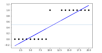
Before that Let me ask you a question why we can't use Linear Regression for classification problems? think about that I will answer here.

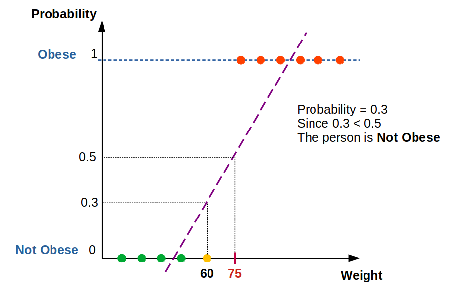
in the image, there are two classes when you're trying to fit a Linear line to classify the data see there is some misclassification to solve this problem researchers created another algorithm which is Logistic Regression. You may think it is why the name is regression. then It is named 'Logistic Regression' because its underlying technology is quite the same as Linear Regression but “Logistic” is taken from the Logit function that is used in this method of classification.

Let us Start

As I said the term Logistics comes from the function Logit

if we take an inverse of the above function, we get:

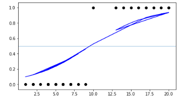
if we plot this in a graph we would get an S-shaped curve this function is called the Sigmoid function the value would lie between 0 to 1.

this sigmoid function is the same as the linear function in Linear Regression

the term Y has a probability ranging from 0 to 1 with this we can classify the data based on some threshold like 0.5 if it is greater than or equal to 0.5 it is 'SPAM' else it is 'NOT SPAM'

In Linear Regression we would train the model until we get a perfect parameter by which we can predict the value accurately similarly Logistic Regression has to undergo training in order to optimize the parameters here the parameters are

How to find error?

In Linear Regression we had cost function like Mean squared error or Mean absolute error likewise logistic function also has cost function which is

This cost function is used to compute the average error between the actual class and the predicted class this is similar to cost function in linear regression but it is adapted according to classification problem.

How to change the value of the parameter?

In Linear regression, we had a Gradient Decent Algorithm to optimize the value of a parameter similarly Logistic regression also uses a Gradient Decent algorithm

• We take a partial derivative of the weight and bias to get the slope of the cost function at each point.

• Based on the slope, gradient descent updates the values for the bias and the set of weights, then re-iterates the training loop over new values.

• This iterative approach is repeated until a minimum error is reached, and gradient descent cannot minimize the cost function any further.

Implementation of Logistic Regression from scratch in python

Function to compute sigmoid

 def sigmoid(z):
    return 1/(1+ np.exp(-z))

Function to compute the hypothesis using sigmoid

def hypothesis(X,theta):
    '''
    X : np.array. shape - (m,n)
    theta : np.array. shape - (n,1)

    return : np.array (m,1)
    '''

    return sigmoid(X.dot(theta))

Function to compute the error

def error(X,Y,theta):
    '''
    X : np.array. shape - (m,n)
    Y : np.array. shape - (m,1)
    theta : np.array. shape - (n,1)

    return : Scalar loss value
    '''

    Y_ = hypothesis(X,theta)
    e = np.mean(Y*np.log(Y_) + (1-Y)*np.log(1-Y_))

    return -e

Function to compute the gradient :

def gradient(X,Y,theta):
    '''
    X : np.array. shape - (m,n)
    Y : np.array. shape - (m,1)
    theta : np.array. shape - (n,1)

    return : np.array (n,1)
    '''

    Y_ = hypothesis(X,theta)
    grad = np.dot(X.T,(Y_ - Y))

    return grad/X.shape[0]

Function for gradient decent

def gradient_descent(X, Y, learning_rate = 0.1, max_iters=100):

    n = X.shape[1]
    theta = np.zeros((n,1))
    error_list = []

    for i in range(max_iters):
        e = error(X,Y,theta)
        error_list.append(e)

        #Gradient descent
        grad = gradient(X,Y,theta)
        theta = theta - learning_rate*grad

    return theta,error_list

Putting it all together:

 def sigmoid(z):
    return 1/(1+ np.exp(-z))


def hypothesis(X,theta):
    '''
    X : np.array. shape - (m,n)
    theta : np.array. shape - (n,1)

    return : np.array (m,1)
    '''

    return sigmoid(X.dot(theta)) 


def gradient(X,Y,theta):
    '''
    X : np.array. shape - (m,n)
    Y : np.array. shape - (m,1)
    theta : np.array. shape - (n,1)

    return : np.array (n,1)
    '''

    Y_ = hypothesis(X,theta)
    grad = np.dot(X.T,(Y_ - Y))

    return grad/X.shape[0]


def gradient_descent(X, Y, learning_rate = 0.1, max_iters=100):

    n = X.shape[1]
    theta = np.zeros((n,1))
    error_list = []

    for i in range(max_iters):
        e = error(X,Y,theta)
        error_list.append(e)

        #Gradient descent
        grad = gradient(X,Y,theta)
        theta = theta - learning_rate*grad

    return theta,error_list

I think you have learned something from the article. If you like my work kindly leave your comments. Happy Learning......