Multiple Linear Regression and Polynomial Regression
3 rd part of the Machine learning brief article series (Ato Z)


Multiple Linear Regression :
In the previous article, we saw Linear Regression (those who are new to the series kindly checkout and continue this) which maps the linear relationship between X and Y, the target variable (Y) which is dependent only on one variable X but in the real world, this does not happen the target variable depends on many variables (Features) for example if you want to determine the price of the house there are many factors which affects the price of the house so want to modify the hypothesis (Equation) which is suitable to handle the multiple input values (or independent values).
The hypothesis of Multiple Linear Regression is
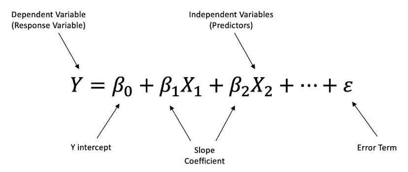
the linear regression hypothesis is modified to suit many independent variables. from the above hypothesis can you infer anything this is nothing but the equation of the plane. In linear regression line tries to fit the data whereas in multiple linear regression plane tries to fit the data
The remaining everything is similar to that of Linear regression let us see the Multiple Linear Regression from scratch in python
def hypothesis(X,theta):
   - '''
    X : np.array. shape - (m,n)
    theta : np.array. shape - (n,1)

    return : np.array (m,1)
    '''

    return X.dot(theta)

def error(X,Y,theta):
    '''
    X : np.array. shape - (m,n)
    Y : np.array. shape - (m,1)
    theta : np.array. shape - (n,1)


    '''

    Y_ = hypothesis(X,theta)
    e = np.sum((Y-Y_)**2)

    return e/(2*X.shape[0])

def gradient(X,Y,theta):
    '''
    X : np.array. shape - (m,n)
    Y : np.array. shape - (m,1)
    theta : np.array. shape - (n,1)

    return : np.array (n,1)
    '''

    Y_ = hypothesis(X,theta)
    grad = np.dot(X.T,(Y_ - Y))

    return grad/X.shape[0]

def gradient_descent(X, Y, learning_rate = 0.1, max_iters=100):

    n = X.shape[1]
    theta = np.zeros((n,1))
    error_list = []

    for i in range(max_iters):
        e = error(X,Y,theta)
        error_list.append(e)

        #Gradient descent
        grad = gradient(X,Y,theta)
        theta = theta - learning_rate*grad

    return theta,error_list
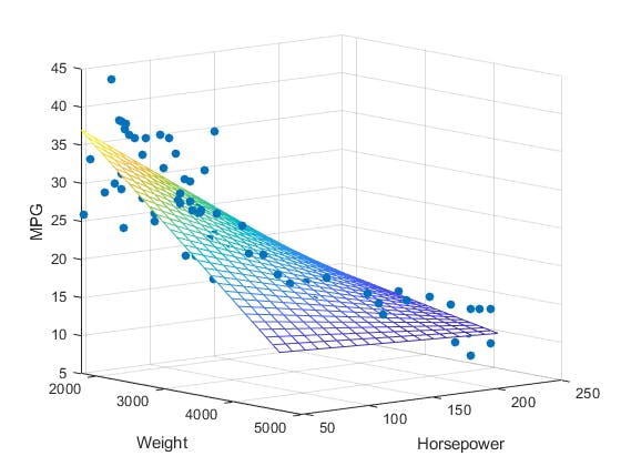
the image of multiple linear regression would be
Polynomial Regression:
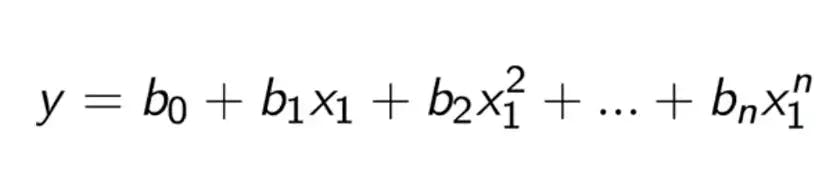
Polynomial Regression forms a relation between the Dependent variable (Y) and the Independent variable as n th degree polynomial This is the formula of Polynomial Regression
Why the need for polynomial regression?
Suppose you have the non-linear dataset where the relationship between X and Y is nonlinear in such scenario polynomial regression will be more helpful.
Let us see the Example of this scenario:
First I import the dependency:
import numpy as np
import pandas as pd
import matplotlib.pyplot as plt
import seaborn as sns
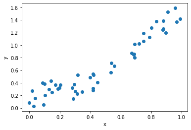
For explaining Polynomial Regression I am going to create dataset which has a non linear relation between X and Y
np.random.seed(1)
X = np.random.rand(50,1)
y = 0.7*(X**5) -  2.1*(X**4) +  2.3*(X**3) +  0.2*(X**2) +  0.3* X +  0.4*np.random.rand(50,1) # no data in world is perfect


fig = plt.figure()
plt.scatter(X, y)
plt.xlabel("x")
plt.ylabel("y")
plt.show()
Let us now predict the value of y using simple Linear regression :
from sklearn.linear_model import LinearRegression
model = LinearRegression().fit(X, y)
outputs = model.predict(X)


fig = plt.figure()
plt.scatter(X, y)
plt.plot(X, outputs, color='red')
plt.xlabel("x")
plt.ylabel("y")
plt.show()
print(model.score(X,y))
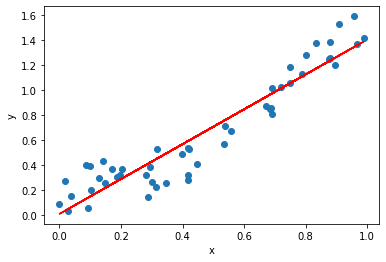
this is the result of Linear regression the score is Approximately 89%
Let us do the same with Polynomial Regression
I am going to create a second degree feature in the dataset and going to predict the result
X_deg2 = np.hstack([X, X**2])

X_deg2.shape
(50, 2)
Again creating a model to predict the improved dataset
model_deg2 = LinearRegression().fit(X_deg2, y)
outputs = model_deg2.predict(X_deg2)


fig = plt.figure()
plt.scatter(X, y)
plt.scatter(X, outputs, color='red')
plt.xlabel("x")
plt.ylabel("y")
plt.show()
print(model_deg2.score(X_deg2,y))
0.937213227713278
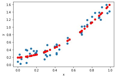
from this image, we can say that this model is somewhat better than previous model the Score of this model is around 93% which is pretty much higher compared to previous model
Similarly we can create third degree polynomial also
X_deg3 = np.hstack([X, X**2, X**3])
model_deg3 = LinearRegression().fit(X_deg3, y)
output = model_deg3.predict(X_deg3)

fig = plt.figure()
plt.scatter(X, y, label="samples")
plt.scatter(X, output, label="prediction")
plt.xlabel("x")
plt.ylabel("y")
plt.legend()
plt.show()
print(model_deg3.score(X_deg3, y))
0.9384895307987052
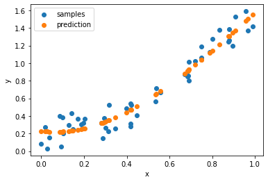
this model also fits perfectly the score is around 94%
As we can see that as the feature increases the score also increases this is only upto certain level. In this way Polynomial Regression can be used for Non Linear dataset.
Another easy method to create polynomial feature on to dataset using Sklearn 's PolynomialFeature method
from sklearn.preprocessing import PolynomialFeatures
poly = PolynomialFeatures(5)
X_poly = poly.fit_transform(X)
X_poly.shape
(50, 6)
This is about Multiple Linear Regression and Polynomial Regression in the next article I will cover Logistic Regression.Happy Learning ....

if you like my work Kindly like and leave your comments....